| Top | Overview | For observers | Gallery | Technical detail | Publications | Data |
|---|
Observing modes
Observers can select one of the three modes (WIDE, HIRES-Y&J)[1] depending on their priority on spectral resolution and wavelength coverage. Three slits of 100 μm-width 140 μm-width, and 200 μm-width are available for WIDE and HIRES-Y&J modes.
[1] Note that the WIDE and HIRES-Y&J modes cannot be switched quickly from one to another during an observing night. to avoid any hardware trouble. To switch the modes, work at the dome is necessary and the exposure of the instrument to light will cause residual signals which may last for a couple of hours.
Mode | WIDE | HIRES-Y | HIRES-J |
|---|---|---|---|
Wavelength coverage | 0.91 - 1.35 μm | 0.96 - 1.11 μm | 1.14 - 1.35 μm |
Spectral resolution | 28,000 | 70,000 [1] | |
Throughput | ~ 50% [2] | ~ 32% [2] | ~ 42% [2] |
Main disperser | Reflective echelle grating | Mosaicked high-blazed echelle grating | |
Array | 1.7 μm cut-off HAWAII-2RG | ||
Size | 1.75 m (L) × 1.07 m (W) × 0.50 m (H) | ||
[1] In the engineering observation on NTT, R∼55,000
[2] Including the throughput of optics and QE of the array.
Wavelength coverages
Overall picture
The wavelength coverages of each echell order for the WIDE, HIRES-Y, and HIRES-J modes are illustrated in the figure below. A model of atmospheric transmission curve is also indicated in the figure.
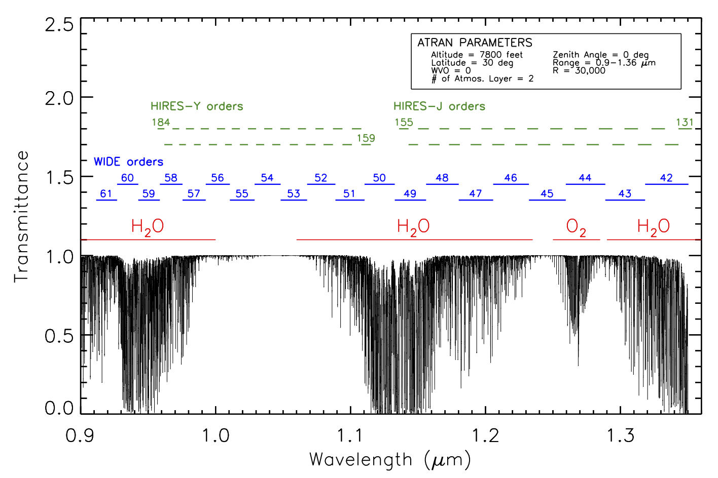
For reference, the observed spectrum of atmospheric absorption with the WIDE mode at Kyoto is available here.
[Click here for details]![]()
Echelle orders projected on the detector
Free spectral ranges
m |
Free spectral range (μm) |
m |
Free spectral range (μm) |
61 |
0.912 – 0.928 |
51 |
1.089 – 1.110 |
60 |
0.928 – 0.942 |
50 |
1.110 – 1.132 |
59 |
0.942 – 0.958 |
49 |
1.132 – 1.156 |
58 |
0.958 – 0.976 |
48 |
1.156 – 1.180 |
57 |
0.976 – 0.992 |
47 |
1.180 – 1.205 |
56 |
0.992 – 1.010 |
46 |
1.205 – 1.232 |
55 |
1.010 – 1.028 |
45 |
1.232 – 1.260 |
54 |
1.028 – 1.048 |
44 |
1.260 – 1.290 |
53 |
1.048 – 1.068 |
43 |
1.290 – 1.319 |
52 |
1.068 – 1.089 |
42 |
1.319 – 1.351 |
m |
Free spectral range (μm) |
m |
Free spectral range (μm) |
184 |
0.957 – 0.962 |
171 |
1.030 – 1.036 |
183 |
0.962 – 0.968 |
170 |
1.036 – 1.042 |
182 |
0.968 – 0.973 |
169 |
1.042 – 1.048 |
181 |
0.973 – 0.978 |
168 |
1.048 – 1.055 |
180 |
0.978 – 0.984 |
167 |
1.055 – 1.061 |
179 |
0.984 – 0.989 |
166 |
1.061 – 1.067 |
178 |
0.989 – 0.995 |
165 |
1.067 – 1.074 |
177 |
0.995 – 1.001 |
164 |
1.074 – 1.080 |
176 |
1.001 – 1.007 |
163 |
1.080 – 1.087 |
175 |
1.007 – 1.012 |
162 |
1.087 – 1.094 |
174 |
1.012 – 1.018 |
161 |
1.094 – 1.101 |
173 |
1.018 – 1.024 |
160 |
1.101 – 1.108 |
172 |
1.024 – 1.030 |
159 |
1.108 – 1.115 |
m |
Free spectral range (μm) |
m |
Free spectral range (μm) |
155 |
1.136 – 1.143 |
142 |
1.239 – 1.248 |
154 |
1.143 – 1.150 |
141 |
1.248 – 1.257 |
153 |
1.150 – 1.158 |
140 |
1.257 – 1.266 |
152 |
1.158 – 1.166 |
139 |
1.266 – 1.275 |
151 |
1.166 – 1.173 |
138 |
1.275 – 1.284 |
150 |
1.173 – 1.181 |
137 |
1.284 – 1.294 |
149 |
1.181 – 1.189 |
136 |
1.294 – 1.303 |
148 |
1.189 – 1.197 |
135 |
1.303 – 1.313 |
147 |
1.197 – 1.205 |
134 |
1.313 – 1.323 |
146 |
1.205 – 1.214 |
133 |
1.323 – 1.333 |
145 |
1.214 – 1.222 |
132 |
1.333 – 1.343 |
144 |
1.222 – 1.231 |
131 |
1.343 – 1.353 |
143 |
1.231 – 1.239 |
Limiting magnitudes
The following table gives estimated limiting magnitudes when the WINERED is attached to the 3.58-meter NTT.
Mode | WIDE | HIRES | ||||
|---|---|---|---|---|---|---|
Slit width [um] | 100 | 140 | 200 | 100 | 140 | 200 |
Slit width [arcsec] | 0.54 | 0.76 | 1.08 | 0.54 | 0.76 | 1.08 |
Slit width [pixel] | 2.0 | 2.8 | 4.0 | 2.0 | 2.8 | 4.0 |
Pixel scale [arcsec/pixel] | 0.27 | |||||
Slit length [arcsec] | 16.34 | |||||
Resolution | 28,000 | 24,000[1] | 18,000 | 68,000[2] | 58,000[3] | 44,000[3] |
z-band limiting magnitude (Vega) | 14.08 | 14.40 | 14.69 | - | - | - |
Y-band limiting magnitude (Vega) | 14.29 | 14.62 | 14.19 | 12.91 | 13.25 | 13.53 |
J-band limiting magnitude (Vega) | 14.40 | 14.73 | 15.02 | 13.03 | 13.35 | 13.64 |
[1] Not measurement, but just expected value.
[2] In the engineering observation on NTT, R∼55,000
[3] Not measurement, but just expected value from an ideal case.
The assumptions made for calculating the above limiting magnitudes are as follows:
- Integration time: 1 hour (900 sec * 4; ABBA sequence)
- S/N: 30
- Point source size: 1.2 arcsec
- Atmospheric transmittance: 0.95
- Throughput of the telescope: 0.55
Estimate of observing time
The following figures show roughly estimated required time as a function of the J-band magnitude. The time is calculated for the point-source observation.
WIDE mode

HIRES-J mode

Overheads
| Action | Time (minutes) |
| Acquisition | 3 [1] |
| Read-out + writing data | 0.2 [2] |
| Nodding to another slit position | 0.5 [1] |
| Offset to sky | 0.2 [1] |
[1] In the case of being installed on Araki telescope.
[2] This is a typical time. Strictly speaking, it depends on the setting of non-destructive reading.
Observing sequences and necessary durations
A typical observing sequence is composed of four integrations at dithered position along the slit (known as an ABBA sequence) for a faint target or three integrations, two with the target within the slit and one for a blank sky (known as an OSO sequence) for a bright target whose PSF gets prominent over a wide area of the slit.
For each sequence, the following formula may be used for estimating a necessary observing time including the overheads. The overheads are estimated for observations with Araki telescope in Koyama observatory at Kyoto Sangyo University, and they may be slightly different when attached to other telescopes. We are going to give realistic estimates of these overheads for observations with NTT 3.6-m telescope after our first observing run(s).
- ABBA: t(integ) + 3 + 4 * 0.2 + 2 * 0.5 [minutes]
- OSO: t(integ) * (3/2) + 3 + 3 * 0.2 + 2 * 0.2 [minutes]
t(integ) is the integration time for a given magnitude.
Detector characteristics
Residual charge
The detector array used in WINERED exhibits a residual charge from bright sources. The residual will typically be ~1% of the originally detected signal.
In order to reduce the influence of the residual charge, bright and faint sources are usually observed at different slit positions [1]. Furthermore, dome flats and comparison lamp spectra will be taken only after observation.
[1] The O position is mainly used for bright sources, while the A and B positions are for faint sources.
Miscellaneous information
- The shortest exposure time is 1.5 sec. In this case, the time to reset, read out and write data is about 10 sec. Therefore, the minimum amount of time between consecutive observation is about 10 sec.
- The linearity limit is around 40000 ADU (or 48000 ADU may be acceptable to ~1.3% deviation) from laboratory experiments.
Data reduction pipeline
We developed the WINERED data-reduction pipeline, which automatically produces 1D spectra from raw data in less than 20 minutes/frame.
Automatic correction for telluric absorption, which is mandatory for infrared spectroscopy, is under development and is planned to be incorporated into the WINERED data-reduction pipeline.
Auxiliary information concerning the WINERED performance
Quality of spectra
The high-sensitivity of WINERED enables us to obtain NIR high-resolution spectra with high signal-to-noise ratio in much shorter time, or bring us to unexplored faint-end by NIR high-resolution spectroscopy. For example, WINERED mounted on a 10-m telescope equipped with AO can be used for the study of the absorption line systems of z > 6 QSOs or GRBs (J > 18 mag).
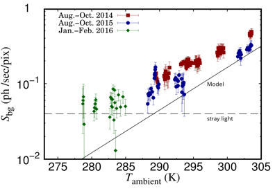
Background
The measured background radiation reaching the array for various the ambient temperatures is shown in the figure below. The difference of plots shows different season. The solid line is a predicted flux with an assumption that the ambient environment is the block body. The dashed lines is the level of measured stray light in the cryostat.
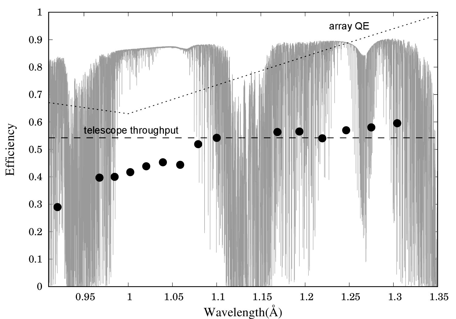
Optical performances
The measurement result of the total throughput of the WIDE-mode (filled circles) that does not include the slit loss is shown in the figure below. The solid line, dashed line, and dotted line are the model of atmospheric transmittance, the asuumed throughput of the 1.3-m Araki telescope, and the quantum efficiency of the array based on measurements by Teledein Inc., respectively.
▲